[COMPANY]

[HEADLINE_CLAIM]

Wind resolved over the real ground at each turbine, carried through to generation and to revenue at your settlement point.

[CTA_LABEL]

(a) Forecast-model cell — 3 km

(b) Resolved cell — 10 m

lower higher

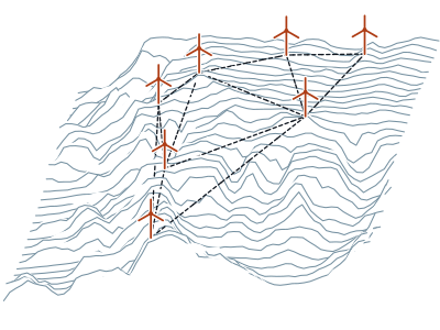
Fig. 1 — One 12 × 6 km site, one elevation dataset, carried at forecast-model resolution on the left of the bar and at ours on the right — drag it. The contour interval is the same on both sides, and the lines are not: on the right they close around the crest and thread the pass; on the left, where the terrain is 4 × 2 numbers, the same iso-height lines run straight past both. The pale lines are air, from the same flow solved over each side of the bar. On the left it crosses the site as though it were flat — the average of a 3 km square has no tops left in it to stand in the way. On the right the same air threads between them, and gathers speed where they pinch it. The rotors mark where that lands: across the 33 machines in the window, the ground the left of the bar puts them on is a median 31 m from the ground they actually stand on, and as much as 125 m. The wind follows the ground on the right. A forecast has the ground on the left.

USGS10m elevation (USGS 3DEP), 10 m native, resampled to 10 m · Big Sampson, Upton County, TX (ERCOT West) · 12 × 6 km, 242 m of relief · 33 turbine positions from the US Wind Turbine Database · elevation and turbine positions are data; the flow is not. It is a depth-averaged potential flow, solved in the page over each side's terrain, drawn to show what the two grounds do to the same air, and it is what turns the rotors — not a forecast, not the reference simulation, and no measured result is shown

elevation contours · 25 m interval · streamlines, equal air flux between neighbours · one three-bladed mark per turbine, centred on its recorded position — a symbol at a fixed size, not a footprint; each turns at the speed of the sketched flow on its side of the bar, which is a property of that sketch and not a predicted wind · each side drawn, and solved, from its own terrain

The problem

Wind error dominates
the day-ahead budget.
The power curve
multiplies it.

The error starts in the wind, and the power curve amplifies it

An operational forecast model resolves the atmosphere in cells about 3 km across. A ridge is narrower than that. So is the pass the wind accelerates through, and so is the eddy that sits in the lee of the crest and takes metres per second off the machines behind it. Inside one cell there is one wind speed.

Day-ahead generation error at a single wind farm is dominated by the wind-speed error inherited from the weather model, not by the conversion from wind to power. The conversion is what makes that error expensive. Through the middle of a turbine's power curve, output goes roughly as the cube of wind speed, so a wind error does not pass through unchanged — it comes out larger.

That is why resolution is not a refinement. A forecast that averages a ridge into its surroundings gets the hub-height wind wrong by a few per cent, and the machine turns that into a much bigger error in megawatt-hours and in settlement.

The approach

Three steps.
The order is real:
each one consumes
the one before it.

Resolve the terrain, predict the machine, price the energy

01

Resolve the terrain

We build the site's elevation at metre scale, mesh it, and resolve the flow over it, with the operational forecast setting the conditions at the edges of the domain. What comes out is a wind field with the ridge speed-up, the pass jet and the lee wake in it — at hub height, at each turbine position.

Fig. 2 — [FIG_TERRAIN_CAPTION]

[FIG_TERRAIN_PROVENANCE]

02

Predict the machine

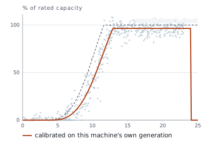
Wind becomes power through a curve calibrated on the turbine's own observed generation rather than the manufacturer's sheet, plus a learned correction for the losses a turbine imposes on the machines downwind of it, trained across multiple wind farms.

Effect of the wake correction on forecast error: [WAKE_IMPROVEMENT].

Fig. 3 — [FIG_GENERATION_CAPTION]

[FIG_GENERATION_PROVENANCE]

03

Price the energy

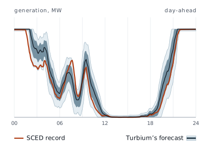
Predicted generation is carried through to the ERCOT nodal price at your settlement point and reported as revenue, over the same horizons as the wind and generation forecasts, so the three line up hour for hour.

Fig. 4 — [FIG_PRICING_CAPTION]

[FIG_PRICING_PROVENANCE]

How it runs

Trained on turbulence.
Never on your site.
The ground is imposed,
not learned.

A model trained on turbulence, not on your site

What runs on every forecast cycle is a pretrained flow model. It was trained on canonical turbulence — generic three-dimensional turbulent motion at a fixed Reynolds number, with no ridge, no wind farm and nobody's ground anywhere in it. It knows how turbulence evolves. It has never seen your site, and it does not need to.

What makes it produce this site's wind is imposed on it, not learned. The site's real elevation enters as an immersed surface with a wall model. The operational forecast is relaxed in at the edges of the domain, and supplies the synoptic situation. A divergence-free projection is applied every step, so mass is conserved rather than approximated. A viscosity correction retunes the model from the Reynolds number it was trained at to the one this site and this weather situation actually have. Every one of those is enforced on the model's output at every step: the learned part carries the interior turbulence, and everything that makes the answer about this ridge on this afternoon is physics, applied afterwards.

That is also why adding a site is a terrain fetch and an inference. There is no training run, no model fitted to your history, and nothing to wait for — coordinates to first forecast is [ONBOARDING_TIME], and each new operational cycle produces a new forecast in [REFRESH_LATENCY]. A site with no usable historical generation still gets a forecast, because history is what the forecast is checked against, never what makes it work.

Refresh latency
[REFRESH_LATENCY]
Coordinates to first forecast
[ONBOARDING_TIME]
(a) Solve cost
[SOLVE_COST]
Agreement
[FIDELITY_VS_LES]
(b) Inference cost
[INFERENCE_COST]

Fig. 5 — The same site and the same hour, twice. On the left the flow is resolved from first principles by the large-eddy simulation; on the right the same hour is produced by the pretrained model that runs operationally. Under each is what it cost: [SOLVE_COST] against [INFERENCE_COST]. Between them is [FIDELITY_VS_LES], how closely the two fields agree — measured on this figure's site and this figure's hour, and a claim about those only. The simulation is the yardstick and not the engine: it costs hours of GPU time for one site in one weather situation, which is exactly why it cannot run on a forecast cycle and exactly why it is worth running to ask whether the fast answer is right.

[FIG_ENGINE_SITE] · [FIG_ENGINE_VALID_TIME] · Large-eddy simulation and pretrained-model inference of one hour over one site · same mesh, same terrain, same operational forecast at the domain edges, same colour scale · site, mesh and valid time as stated with the figure · [SOLVE_COST] and [INFERENCE_COST] measured on the same hardware · one site and one hour, not an average over sites or hours · no market data and no generation forecast appears here

Results

Measured against
ERCOT 60-day SCED
generation data.

Validated against ERCOT 60-day SCED generation data

The comparison below is against real five-minute generation from real Texas wind farms, published by ERCOT in its 60-day SCED disclosure — not against another model and not against synthetic cases.

Over [VALIDATION_SITES] and [VALIDATION_PERIOD], [VALIDATION_N] samples, the day-ahead generation forecast scores [METRIC_OURS]. That is the standard forecast, on sites the model was not fitted to.

Fig. 6 — [FIG_RESULTS_CAPTION]

[FIG_RESULTS_PROVENANCE]

[METRIC_NAME], normalized two ways
Forecast [METRIC_NAME] Skill vs.
persistence
% of installed
capacity
% of actual
energy
[COMPANY] — terrain-resolving forecast [NRMSE_CAPACITY] [NRMSE_ENERGY] [SKILL_VS_PERSISTENCE]
HRRR, interpolated to hub height [METRIC_HRRR] [METRIC_HRRR_ENERGY]
Persistence [METRIC_PERSISTENCE] [METRIC_PERSISTENCE_ENERGY]
  1. Normalization: [NORMALIZATION]. Error as a fraction of installed capacity and as a fraction of the energy actually produced differ by several times; quoting only the first is the standard way to look good, so both are given.
  2. Reference: ERCOT 60-day SCED generation data, [VALIDATION_SITES], [VALIDATION_PERIOD], [VALIDATION_N] samples.

The fastest way to know whether this helps is to run it on your site.

[CTA_LABEL] [CONTACT_EMAIL]